On Schedule only supports a single loan, the development loan. You draw from it as needed to meet project costs, and you pay the interest each month. Normally, you would apply a certain percentage of your unit sale proceeds toward repaying the loan. See The Development Loan in On Schedule for more information.
But what if you have some other financing, such as a regular amortized loan? This article will show you how to model an amortized loan in On Schedule. The steps here will take a bit of time, and they require some fluency in Excel. If you are an Excel novice, you may prefer to have us do this for you as a customization.
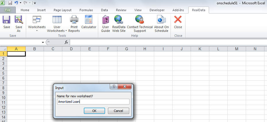
First, add a user worksheet by going to User Worksheets in the RealData menu, and choosing Add. You will then be prompted for the name of the worksheet. You can call it “Amortized Loan.”
In the new worksheet, set up some cells where you can enter the parameters of the loan, and then build the amortization table. Here we are following the convention that data entry cells (Loan Amount, Interest Rate and Term in Months) are in blue font. We are also assuming the interest rate is fixed.
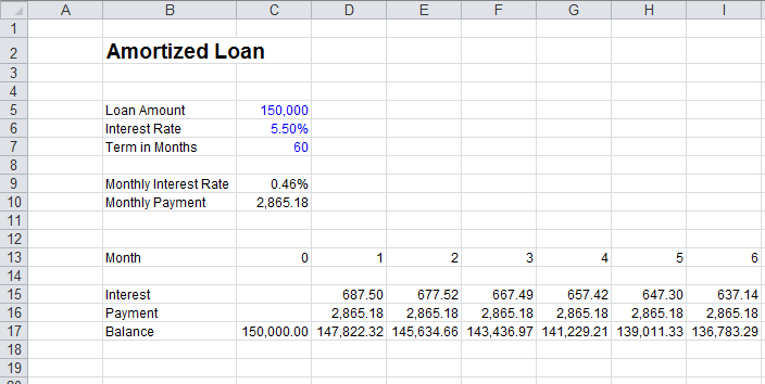
Here are the formulas:
- C9: =C6/12
- C10: =ROUNDUP(PMT(C9,C7,-C5),2)
- C17: =C5
- D13: =C13+1
- D15: =ROUND(C17*$C$9,2)
- D16: =MIN($C$10,C17+D15)
- D17: =C17+D15-D16
You then propagate the formulas in D13:D17 to the right, enough columns to cover the term of the loan (in this case, 60 months). To do this, select D13:D17, do Copy, then select E13:BK17 and do Paste.
Now go back to the Development & Absorption worksheet, and find two unused categories of soft costs. In this example, we are using rows 46 and 47.
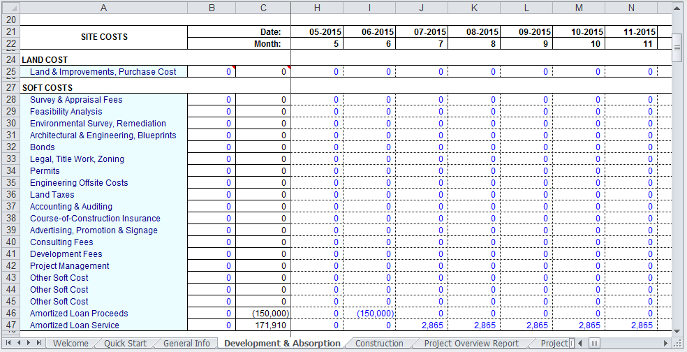
Enter the label “Amortized Loan Proceeds” in cell A46. In the month when you will be taking out the loan, enter a formula to retrieve the amount of the loan from the user worksheet, and negate it. In this example, you are taking out the loan in month 6. Enter the label “Amortized Loan Service” in cell A47. In the first month after you take out the loan, enter a formula to retrieve the first monthly payment from the user worksheet. Here are the formulas:
- I46: =-‘Amortized Loan’!C5
- J47: =’Amortized Loan’!D16
Then propagate the formula in J47 to the right, enough columns to cover the term of the loan (in this case, 60 months). To do this, select J47, do Copy, then select I47:BQ47, and do Paste.
If soft cost categories are scarce, you could combine rows 46 and 47. Notice that Amortized Loan Proceeds is a positive cash flow, and we are representing it as a negative soft cost. Another option is to enter it in row 116 (Rental Revenue) as a positive amount. But in that case, you should probably enter 0.00% for the corresponding month in row 117.