articles
How to Build an Income-Property Pro Forma: A Step-by-Step Flowchart Guide
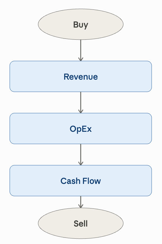
I’ve done a good deal of teaching about the process of underwriting real estate investments, particularly income-producing properties. I’ve seen some good approaches and some not so good.
Chances are, if you’re doing a pro forma workup, it’s not just for your own benefit, but also to convey your point of view to a third party. You might be telling the seller or a potential lender, “Here’s what I think is a fair price for this property, and why.”